Difference between revisions of "Tutorial: Open a model to browse"
DKontotasiou (talk | contribs) |
|||
| (154 intermediate revisions by 8 users not shown) | |||
| Line 1: | Line 1: | ||
| − | < | + | [[Category:Analytica Tutorial]] |
| − | This | + | [[Category: Rent vs. Buy model]] |
| − | + | <breadcrumbs>Analytica Tutorial > {{PAGENAME}}</breadcrumbs> | |
| − | + | {{ReleaseBar}} | |
| − | + | <span style="font-size: large; font-weight: bold;">This simple tutorial shows you how to explore a small Analytica model.</span> | |
| − | |||
| − | == | + | <span style="font-size: large;">It will help you get a feel for how Analytica works!</span> |
| − | + | ||
| − | # | + | |
| − | # After Analytica starts, select '''File''' → '''Open''' from the menu. | + | ==Open the Rent vs. Buy model== |
| + | Follow these steps: | ||
| + | |||
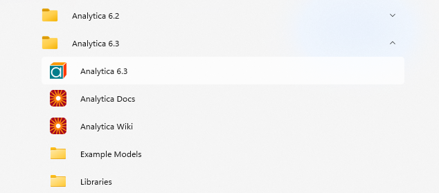
| + | # You start Analytica like any Windows application: For example, click the '''Start''' button on the Windows taskbar. Click {{Release|5.0|6.3|'''All Programs'''}}{{Release|6.4||'''All Apps'''}} → '''Analytica {{#svarget:anarelease|4.6}}''' → '''Analytica {{#svarget:anarelease|4.6}}'''. <br>{{Release||4.6|[[File:Chapter 1.1.png|300px]]}}{{Release|5.0|5.4|[[File:Launch Ana5.0 from Start Menu.png|300px]]}}{{Release|6.0|6.3|[[File:Launch Ana6.0 from Start Menu.png]]}}{{Release|6.4||[[image:Launch Ana6.4 from Start Menu.png]]}} | ||
| + | # After Analytica starts, {{Release||4.6| | ||
| + | select '''File''' → '''Open''' from the menu. | ||
# <br> [[File:Chapter 1.2a.png]] | # <br> [[File:Chapter 1.2a.png]] | ||
# Open the Rent vs. Buy model. <br> [[File:Chapter 1.2b.png]] <br> Analytica reads in the Rent vs. Buy model. | # Open the Rent vs. Buy model. <br> [[File:Chapter 1.2b.png]] <br> Analytica reads in the Rent vs. Buy model. | ||
| + | }}{{Release|5.0|5.4| | ||
| + | select the ''Rent vs. Buy Example'' on the [[Intro screen]].<br /> | ||
| + | [[File:Open Buy vs Rent Example.png]] | ||
| + | }}{{Release|6.0|6.3|select the ''Rent vs. Buy Example'' on the [[Intro screen]].<br /> | ||
| + | {{CalloutAnnotationBlock|[[File:Open Buy vs Rent Example6.0.png]]|{{CalloutAnnotation|Click the Rent vs Buy<br /> | ||
| + | Example model|v=451|pt=34,531|path=b(*,531)}}}}}} | ||
| + | {{Release|6.4||select the ''Rent vs. Buy Example'' on the [[Intro screen]].<br /> | ||
| + | {{CalloutAnnotationBlock|[[File:Open Buy vs Rent Example6.4.png|640px]]|{{CalloutAnnotation|Click the Rent vs Buy<br /> | ||
| + | example model|v=300|pt=38,380|path=b(*,380)}}}}}} | ||
| − | == | + | ==The Diagram window== |
| − | When you open a model, Analytica first displays a top-level | + | When you open a model, Analytica first displays a top-level [[Diagram window]]. A diagram is a graphical user interface that displays user inputs and outputs, influence diagrams, pictures, and other visual elements and controls, and is designed by the author of the model. The ''Rent vs. Buy'' model diagram shows several input variables that affect the trade-offs between renting and buying, '''Normal''' distribution buttons, a '''Calc''' button, and a node labeled Model. |
| − | [[ | + | {{Release|4.6|6.3|{{CalloutAnnotationBlock|[[image:Chapter 1.3.png]]| |
| + | {{CalloutAnnotation| | ||
| + | Normal distrib. button|v=110|pt=215,129|path=r-}} | ||
| + | {{CalloutAnnotation| | ||
| + | User input |v=170|pt=215,175|path=r-}} | ||
| + | {{CalloutAnnotation| | ||
| + | Model node|v=230|pt=276,230|path=r-}} | ||
| + | {{CalloutAnnotation| | ||
| + | Calc button to see results|v=268|pt=412,262|path=r-}} | ||
| + | }}}}{{Release|6.4||{{CalloutAnnotationBlock|[[image:Chapter 1.3v2.png]]| | ||
| + | {{CalloutAnnotation| | ||
| + | User input |v=125|pt=331,130|path=r-}} | ||
| + | {{CalloutAnnotation| | ||
| + | Normal distrib. button|v=290|pt=331,295|path=r-}} | ||
| + | {{CalloutAnnotation| | ||
| + | Calc button to see results|v=430|pt=331,447|path=r-}} | ||
| + | {{CalloutAnnotation| | ||
| + | Model node|v=500|pt=200,515|path=r-}} | ||
| + | }}}} | ||
| + | This top-level diagram is an end-user interface to the model itself, which is contained in the Model node. In this chapter, you use only the interface in this top level diagram; in the following chapters you will explore the model in more depth. | ||
| − | + | Across the top of the screen is a [[toolbar|horizontal palette of buttons]]. This is called the '''''tools palette'''''. | |
| − | + | :{{Release||4.6|[[File:Chapter 1.4.png]]}} | |
| + | {{Release|5.0|| | ||
| + | {{CalloutAnnotationBlock|[[image:BrowseToolOnToolbar5.0.png]]| | ||
| + | {{CalloutAnnotation|The browse tool|v=0|pt=267,33|path=bD10-}}}} | ||
| + | }} | ||
| − | [[File:Chapter 1. | + | When you first open the ''Rent vs. Buy'' model, the '''browse tool''' is highlighted on the palette. With the browse tool selected, the cursor looks like a hand [[File:Chapter 1.5.png|32px]] when it is over the diagram. The browse tool allows you to calculate the model, change input values, and examine — but not change — the structure of the model. <!-- [DP - need the edit mode for some of this page ] In this chapter, you only use the browse tool.--> |
| − | + | ==Access Help Resources== | |
| − | + | At any time, you can press the ''F1'' key on the keyboard or use the '''Help''' menu to access Analytica’s help resources online. This menu includes links to this [[Analytica Tutorial|Tutorial]], the [[Analytica User Guide|User Guide]] and much more tips and reference material on this [[Analytica Docs]]. | |
| − | At any time, you can press the F1 key on the keyboard or use the Help | ||
| − | == | + | ==Compute output values== |
| − | |||
| − | + | In the ''Rent vs. Buy'' model, the output value of interest is at the bottom, ''Present value of buying and renting''. | |
| − | [[ | + | {{Release|4.6|6.3|{{CalloutAnnotationBlock|[[image:Chapter 1.3.png]]| |
| + | {{CalloutAnnotation| | ||
| + | Click the '''Calc''' button to compare the present value of buying and renting.|v=200|pt=413,265|path=bD20-|n=1}} | ||
| + | }}}}{{Release|6.4||{{CalloutAnnotationBlock|[[image:Chapter 1.3v2.png]]| | ||
| + | {{CalloutAnnotation| | ||
| + | Click the '''Calc''' button to compare the present value of buying and renting.|v=350|pt=331,447|path=bD20-|n=1}} | ||
| + | }}}} | ||
| − | The output value displays in a | + | The output value displays in a [[Result window]]. This '''Result''' window shows a graph of two '''''probability density''''' curves, one for buying and one for renting. In a probability density graph, the units of the vertical scale are chosen so that the total area under each curve is 1 (100%). 25μ corresponds to 25 x 10-6 or 0.000025. |
| − | + | <tip>Numerical suffixes like μ and K are used extensively throughout Analytica. A quick reference for these suffixes is given in [[Number formats]] .</tip> | |
| − | Numerical suffixes like μ and K are used extensively throughout Analytica. A quick reference for these suffixes is given | ||
| − | |||
| − | [[File:Chapter 1.7.png]] | + | :{{Release|4.6|6.3|[[File:Chapter 1.7.png]]}}{{Release|6.4||[[File:Chapter 1.7v2.png]]}} |
| − | Since the graph is of probability densities, both buying and renting have probabilistic, or uncertain, inputs. The probability density graph for each appear to be bell-shaped curves ( | + | Since the graph is of probability densities, both buying and renting have probabilistic, or uncertain, inputs. The probability density graph for each appear to be bell-shaped curves ([[normal]] distribution), although they appear a bit “noisy.” |
The graphs show that the cost of renting, given the model’s inputs, are between about $105,000 and $155,000 (the negative numbers mean cost — cash flowing out), while the cost of buying is between $115,000 and a gain of $75,000. | The graphs show that the cost of renting, given the model’s inputs, are between about $105,000 and $155,000 (the negative numbers mean cost — cash flowing out), while the cost of buying is between $115,000 and a gain of $75,000. | ||
| − | [[ | + | {{Release|4.6|6.3|{{CalloutAnnotationBlock|[[image:Chapter 1.8.png]]| |
| + | {{CalloutAnnotation| | ||
| + | Click the '''Diagram''' window to bring it to the front.|v=40|pt=30,140|path=b!|n=+}} | ||
| + | }}}}{{Release|6.4||{{CalloutAnnotationBlock|[[image:Chapter 1.8v2.png]]| | ||
| + | {{CalloutAnnotation| | ||
| + | Click the '''Diagram''' window to bring it to the front.|v=40|pt=30,140|path=b!|n=+}} | ||
| + | }}}} | ||
'''''Note''': Your results can vary slightly, since the model is generating random inputs based on a normal distribution for the uncertainty of the rate of inflation and for the appreciation rate.'' | '''''Note''': Your results can vary slightly, since the model is generating random inputs based on a normal distribution for the uncertainty of the rate of inflation and for the appreciation rate.'' | ||
| − | Click the model | + | Click the model [[Diagram window]] to bring it to the front. Notice that the button next to ''Costs of buying and renting'' has changed to '''Result'''. The '''Result''' button indicates that the value has been computed; clicking the '''Result''' button re-displays the computed values. |
| − | [[ | + | {{Release|4.6|6.3|{{CalloutAnnotationBlock|[[image:Chapter 1.9.png]]| |
| + | {{CalloutAnnotation| | ||
| + | The '''Calc''' button has changed to '''Result'''.|v=220|pt=413,265|path=bD15-}} | ||
| + | }}}}{{Release|6.4||{{CalloutAnnotationBlock|[[image:Chapter 1.9v2.png]]| | ||
| + | {{CalloutAnnotation| | ||
| + | The '''Calc''' button has changed to '''Result'''.|v=400|pt=331,447|path=bD20-}} | ||
| + | }}}} | ||
| − | == | + | ==Examine definition types in user input nodes== |
| − | |||
| − | + | When you enter a value into a user input, you need to enter a value that is compatible with it's definition type. See more here...[[The_Expression_popup_menu|Expression popup menu]]. | |
| − | [[File: | + | Click the '''Time horizon''' node.<br/> |
| + | Press ''F4'' to bring up the object window.<br/> | ||
| + | {{Release|4.6|6.3|{{CalloutAnnotationBlock|[[File:Chapter1 8a.png]]| | ||
| + | {{CalloutAnnotation| | ||
| + | Click the Variable ''Time horizon'', then press F4.|v=53|pt=44,90|n=1}} | ||
| + | }}}}{{Release|6.4||{{CalloutAnnotationBlock|[[File:Chapter1 8av2.png]]| | ||
| + | {{CalloutAnnotation| | ||
| + | Click the Variable ''Time horizon'', then press F4.|v=89|pt=47,125|n=1}} | ||
| + | }}}} | ||
| − | + | Press ''F9'' to enter edit mode (otherwise the expression popup menu is disabled). | |
| − | |||
| − | |||
| − | + | Click on the Expression popup menu (here it has a numeric icon, since this input is restricted to numbers only). <br/> | |
| + | Note that Number only is selected. If you attempt enter text into the input node you will get a warning.<br/> | ||
| + | {{Release|4.6|6.3|{{CalloutAnnotationBlock|[[File:Chapter1 8b.png]]| | ||
| + | {{CalloutAnnotation| | ||
| + | Click on the Expression popup menu - Note that Number only is selected. |v=150|pt=280,263|path=rR10!|n=2}} | ||
| + | }}}}{{Release|6.4||{{CalloutAnnotationBlock|[[File:Chapter1 8bv2.png]]| | ||
| + | {{CalloutAnnotation| | ||
| + | Click on the Expression popup menu - Note that Number only is selected. |v=180|pt=220,293|path=rR10!|n=2}} | ||
| + | }}}} | ||
| − | + | Press ''F8'' to go back to Browse mode. | |
| − | [[File: | + | Close the object window - click the object window icon at the top left of the object window and select '''Close''' from the popup menu. <br/> |
| + | {{Release|4.6|6.3|{{CalloutAnnotationBlock|[[File:Chapter1 8c.png]]| | ||
| + | {{CalloutAnnotation| | ||
| + | Click on the Object window icon. |v=130|pt=212,156|n=3}} | ||
| + | {{CalloutAnnotation| | ||
| + | Select ''Close''. |v=317|pt=231,335|n=4}} | ||
| + | }}}}{{Release|6.4||{{CalloutAnnotationBlock|[[File:Chapter1 8cv2.png]]| | ||
| + | {{CalloutAnnotation| | ||
| + | Click on the Object window icon. |v=145|pt=110,171|n=3}} | ||
| + | {{CalloutAnnotation| | ||
| + | Select ''Close''. |v=298|pt=110,315|n=4}} | ||
| + | }}}} | ||
| − | + | ==Change input values and recompute results== | |
| − | + | Now you will change some input values to the model and recompute the rent vs. buy comparison. You will change the values of ''Time horizon'', ''Monthly rent'', and ''Buying price''. | |
| − | + | {{Release|4.6|6.3|{{CalloutAnnotationBlock|[[image:Chapter 1.9.png]]| | |
| + | {{CalloutAnnotation| | ||
| + | Click the box next to ''Time horizon''. Change the value to '''''7''''' and press ''Alt+Enter''.|v=50|pt=220,64|path=tU20-|n=1}} | ||
| + | }}}}{{Release|6.4||{{CalloutAnnotationBlock|[[image:Chapter 1.9v2.png]]| | ||
| + | {{CalloutAnnotation| | ||
| + | Click the box next to ''Time horizon''. Change the value to '''''7''''' and press ''Alt+Enter''.|v=127|pt=331,130|path=tU20-|n=1}} | ||
| + | }}}} | ||
| − | + | <tip>The main Enter key and the numeric keypad Enter key are not interchangeable. They have different functions in Analytica. Alt+Enter is equivalent to the numeric keypad Enter key.</tip> | |
| − | + | As soon as you change an input, the '''Result''' button changes to a '''Calc''' button, indicating that ''Present value of buying and renting'' needs to be recomputed. | |
| − | [[ | + | {{Release|4.6|6.3|{{CalloutAnnotationBlock|[[image:Chapter 1.10.png]]| |
| + | {{CalloutAnnotation| | ||
| + | Click the box next to ''Monthly rent''. Change the value to '''''1400''''' and press ''Alt+Enter''.|v=170|pt=220,174|path=r-|n=+}} | ||
| + | }}}}{{Release|6.4||{{CalloutAnnotationBlock|[[image:Chapter 1.10v2.png]]| | ||
| + | {{CalloutAnnotation| | ||
| + | Click the box next to ''Monthly rent''. Change the value to '''''1400''''' and press ''Alt+Enter''.|v=127|pt=331,160|path=r-|n=+}} | ||
| + | }}}} | ||
| − | == | + | {{Release|4.6|6.3|{{CalloutAnnotationBlock|[[image:Chapter 1.11.png]]| |
| − | + | {{CalloutAnnotation| | |
| + | Click the box next to ''Buying price''. Change the value to '''''180K''''' (or 180000) and press ''Alt+Enter''.|v=130|pt=510,65|path=tU100-|n=+}} | ||
| + | }}}}{{Release|6.4||{{CalloutAnnotationBlock|[[image:Chapter 1.11v2.png]]| | ||
| + | {{CalloutAnnotation| | ||
| + | Click the box next to ''Buying price''. Change the value to '''''180K''''' (or 180000) and press ''Alt+Enter''.|v=150|pt=331,197|path=r-|n=+}} | ||
| + | }}}} | ||
| − | + | Now you are ready to recompute to see the new results. | |
| − | + | {{Release|4.6|6.3|{{CalloutAnnotationBlock|[[image:Chapter 1.12.png]]| | |
| − | [[ | + | {{CalloutAnnotation| |
| − | + | Click the '''Calc''' button to compute the comparison of the costs of buying to renting.|v=140|pt=413,265|path=bD20-|n=+}} | |
| − | + | }}}} | |
| − | < | + | <!--Don't know what this is |
| − | + | {{Release|4.6|6.3|{{CalloutAnnotationBlock|[[image:Chapter 1.12v2.png]]| | |
| − | + | {{CalloutAnnotation| | |
| − | + | Click the '''Calc''' button to compute the comparison of the costs of buying to renting.|v=430|pt=331,447|path=r-|n=+}} | |
| − | [[ | + | }}}}--> |
| − | |||
| − | |||
| − | |||
| − | |||
| − | + | The graphs show that the cost of renting, given these changed inputs, is between $90,000 and $120,000, while the cost of buying is between $135,000 and a gain of $70,000. | |
| − | |||
| − | + | {{Release|4.6|6.3|{{CalloutAnnotationBlock|[[image:Chapter 1.13.png]]| | |
| + | {{CalloutAnnotation| | ||
| + | Click the '''Diagram''' window to bring it to the front.|v=80|pt=43,232|path=b!|n=+}} | ||
| + | }}}}{{Release|6.4||{{CalloutAnnotationBlock|[[image:Chapter 1.13v2.png]]| | ||
| + | {{CalloutAnnotation| | ||
| + | Click the '''Diagram''' window to bring it to the front.|v=40|pt=30,140|path=b!|n=+}} | ||
| + | }}}} | ||
| − | + | ==Save your model== | |
| + | If you want to save changes to your model, you can do so at this point. (For instructions on quitting without saving, see the next section). | ||
| − | + | Since the Analytica folder in Program files is not writable by default to a non admin user, you have to be running Analytica as an admin to be able to save over the original model file. | |
| − | + | {{CalloutAnnotationBlock|[[image:Chapter 1.30.png]]|{{CalloutAnnotation| | |
| + | Click '''Save''' from the File menu.|v=220|pt=30,180}}}} | ||
| − | + | If you wish to save your model as a different file, so that you do not change the original model, select '''Save As''' from the [[File menu]]. | |
| − | + | ==Quit Analytica== | |
| − | + | When you have finished using a model, you might want to quit Analytica. | |
| − | |||
| − | |||
| − | |||
| − | |||
| − | |||
| − | |||
| − | |||
| − | |||
| − | |||
| − | |||
| − | |||
| − | |||
| − | |||
| − | |||
| − | |||
| − | |||
| − | |||
| − | |||
| − | |||
| − | |||
| − | Analytica | ||
| − | |||
| − | |||
| − | |||
| − | |||
| − | [[ | + | {{CalloutAnnotationBlock|[[image:Chapter 1.33.png]]|{{CalloutAnnotation| |
| + | Click '''Exit''' from the File menu.|v=370|pt=20,540}}}} | ||
| − | + | == Summary == | |
| − | + | You have now opened an Analytica model, calculated and viewed the results, changes input values and probability distributions, and displayed the uncertain results in several ways. These are the basic techniques for using any quantitative model. | |
| − | [[ | + | After you create your own models, you might want to give them a top-level input and output diagram like the one used in this chapter. For information about customizing a model for end users, see [[Creating Interfaces for End Users]] in the [[Analytica User Guide]]. |
| − | The | + | The next Tutorial page, shows how to navigate the details of the Rent vs. Buy model, exploring its structure and contents. |
| − | + | ==Notes== | |
| + | <references/> | ||
| − | + | ==See Also== | |
| − | + | <div style="column-count:2;-moz-column-count:2;-webkit-column-count:2"> | |
| − | + | * [https://www.analyticacloud.com/acp/Client/AcpClient.aspx?inviteId=3&inviteCode=221703&subName=acp%20demos Play the Rent vs. Buy model in Analytica Cloud Player] | |
| − | + | * [https://www.youtube.com/watch?v=GQV0dnDN0Q0 Using the Rent vs. Buy Model] (an explanatory video on YouTube) | |
| − | + | * [[Tutorial videos]] | |
| − | + | * [[To open or exit a model]] | |
| − | + | * [[Create and save a model]] | |
| − | + | * [[Tutorial: Create a model]] | |
| − | + | * [[Example Models]] | |
| − | + | * [[Example Models and Libraries]] | |
| − | + | * [[Diagram window]] | |
| − | + | * [[Help menu and documentation]] | |
| − | + | * [[User input nodes and user output nodes]] | |
| − | + | * [[Expressing Uncertainty]] | |
| − | + | * [[Uncertainty Setup dialog]] | |
| − | + | * [[Uncertainty view of a result]] | |
| − | + | * [https://youtu.be/d7NzEARJzIg User interfaces (UI) basics] video tutorial | |
| − | + | </div> | |
| − | |||
| − | |||
| − | |||
| − | |||
| − | |||
| − | |||
| − | |||
| − | |||
| − | |||
| − | |||
| − | |||
| − | |||
| − | [[ | ||
| − | |||
| − | |||
| − | |||
| − | |||
| − | |||
| − | |||
| − | + | <footer>Analytica Tutorial/ {{PAGENAME}} / Tutorial: Reviewing a model</footer> | |
Latest revision as of 05:26, 13 February 2025
| Release: |
• 4.6 • 5.0 • 5.1 • 5.2 • 5.3 • 5.4 • • 6.0 • 6.1 • 6.2 • 6.3 • 6.4 • 6.5 • 6.6 |
|---|
This simple tutorial shows you how to explore a small Analytica model.
It will help you get a feel for how Analytica works!
Open the Rent vs. Buy model
Follow these steps:
- You start Analytica like any Windows application: For example, click the Start button on the Windows taskbar. Click All Apps → Analytica 6.5 → Analytica 6.5.
- After Analytica starts,

select the Rent vs. Buy Example on the Intro screen.

example model
The Diagram window
When you open a model, Analytica first displays a top-level Diagram window. A diagram is a graphical user interface that displays user inputs and outputs, influence diagrams, pictures, and other visual elements and controls, and is designed by the author of the model. The Rent vs. Buy model diagram shows several input variables that affect the trade-offs between renting and buying, Normal distribution buttons, a Calc button, and a node labeled Model.

This top-level diagram is an end-user interface to the model itself, which is contained in the Model node. In this chapter, you use only the interface in this top level diagram; in the following chapters you will explore the model in more depth.
Across the top of the screen is a horizontal palette of buttons. This is called the tools palette.
When you first open the Rent vs. Buy model, the browse tool is highlighted on the palette. With the browse tool selected, the cursor looks like a hand ![]() when it is over the diagram. The browse tool allows you to calculate the model, change input values, and examine — but not change — the structure of the model.
when it is over the diagram. The browse tool allows you to calculate the model, change input values, and examine — but not change — the structure of the model.
Access Help Resources
At any time, you can press the F1 key on the keyboard or use the Help menu to access Analytica’s help resources online. This menu includes links to this Tutorial, the User Guide and much more tips and reference material on this Analytica Docs.
Compute output values
In the Rent vs. Buy model, the output value of interest is at the bottom, Present value of buying and renting.
The output value displays in a Result window. This Result window shows a graph of two probability density curves, one for buying and one for renting. In a probability density graph, the units of the vertical scale are chosen so that the total area under each curve is 1 (100%). 25μ corresponds to 25 x 10-6 or 0.000025.

Since the graph is of probability densities, both buying and renting have probabilistic, or uncertain, inputs. The probability density graph for each appear to be bell-shaped curves (normal distribution), although they appear a bit “noisy.”
The graphs show that the cost of renting, given the model’s inputs, are between about $105,000 and $155,000 (the negative numbers mean cost — cash flowing out), while the cost of buying is between $115,000 and a gain of $75,000.

Note: Your results can vary slightly, since the model is generating random inputs based on a normal distribution for the uncertainty of the rate of inflation and for the appreciation rate.
Click the model Diagram window to bring it to the front. Notice that the button next to Costs of buying and renting has changed to Result. The Result button indicates that the value has been computed; clicking the Result button re-displays the computed values.

Examine definition types in user input nodes
When you enter a value into a user input, you need to enter a value that is compatible with it's definition type. See more here...Expression popup menu.
Click the Time horizon node.
Press F4 to bring up the object window.

Press F9 to enter edit mode (otherwise the expression popup menu is disabled).
Click on the Expression popup menu (here it has a numeric icon, since this input is restricted to numbers only).
Note that Number only is selected. If you attempt enter text into the input node you will get a warning.

Press F8 to go back to Browse mode.
Close the object window - click the object window icon at the top left of the object window and select Close from the popup menu.

Change input values and recompute results
Now you will change some input values to the model and recompute the rent vs. buy comparison. You will change the values of Time horizon, Monthly rent, and Buying price.
As soon as you change an input, the Result button changes to a Calc button, indicating that Present value of buying and renting needs to be recomputed.


Now you are ready to recompute to see the new results.
The graphs show that the cost of renting, given these changed inputs, is between $90,000 and $120,000, while the cost of buying is between $135,000 and a gain of $70,000.

Save your model
If you want to save changes to your model, you can do so at this point. (For instructions on quitting without saving, see the next section).
Since the Analytica folder in Program files is not writable by default to a non admin user, you have to be running Analytica as an admin to be able to save over the original model file.

If you wish to save your model as a different file, so that you do not change the original model, select Save As from the File menu.
Quit Analytica
When you have finished using a model, you might want to quit Analytica.

Summary
You have now opened an Analytica model, calculated and viewed the results, changes input values and probability distributions, and displayed the uncertain results in several ways. These are the basic techniques for using any quantitative model.
After you create your own models, you might want to give them a top-level input and output diagram like the one used in this chapter. For information about customizing a model for end users, see Creating Interfaces for End Users in the Analytica User Guide.
The next Tutorial page, shows how to navigate the details of the Rent vs. Buy model, exploring its structure and contents.
Notes
See Also
- Play the Rent vs. Buy model in Analytica Cloud Player
- Using the Rent vs. Buy Model (an explanatory video on YouTube)
- Tutorial videos
- To open or exit a model
- Create and save a model
- Tutorial: Create a model
- Example Models
- Example Models and Libraries
- Diagram window
- Help menu and documentation
- User input nodes and user output nodes
- Expressing Uncertainty
- Uncertainty Setup dialog
- Uncertainty view of a result
- User interfaces (UI) basics video tutorial
Enable comment auto-refresher