The Sensitivity Analysis Library

The Sensitivity Analysis Library provides functions that help you create sensitivity analyses of models containing array-valued inputs.

The functions in this library allow you to compute the sensitivity of a result to each cell of each array-valued uncertain input. It is similar to Make Importance (on the Object menu), except that Make Importance varies each chance array input as a whole, while the functions in this library vary each individual cell of array-valued input variables.

Download

To use, download the library from Sensitivity Analysis Library.

The Sensitivity Functions Examples.ana model demonstrates the use of this library.

Webinar on Using It

You can watch recordings of two webinars that cover the topic of setting up and graphing sensitivity analyses:

The first webinar is a pre-requisite for the second. The last part of the second webinar introduces this library and demonstrates its usage.

Abstracts of these talks are at Analytica User Group/Past Topics.

What is Computed

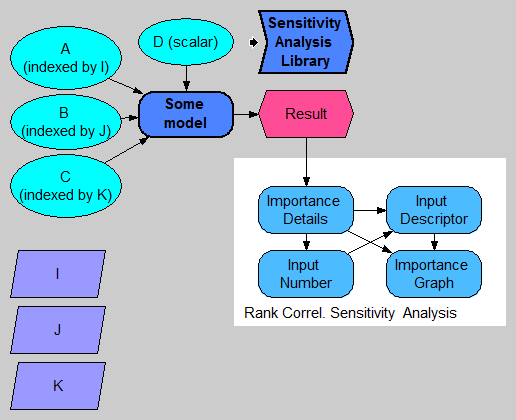
The following diagram depicts a model having four uncertain inputs, A, B, C, and D, of which A, B, and C are array-valued with various indexes (pay attention to the top-left). The model computes Result.

Because we are considering every cell of every input array, there could in general be a huge number of inputs to depict. It is therefore of value to direct our attention only to the few inputs having the greatest sensitivity.

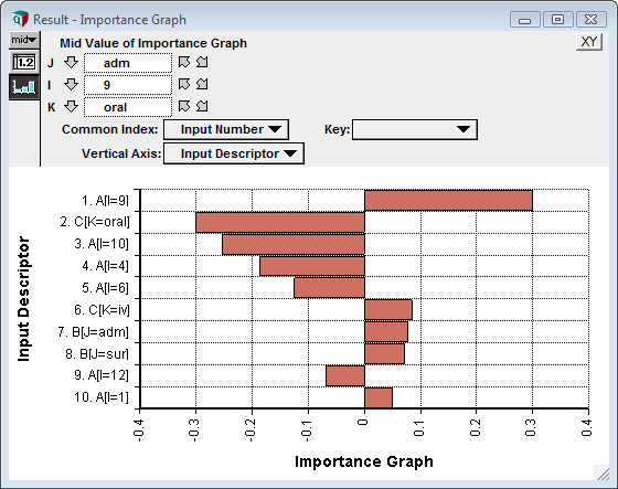
The Sensitivity Analysis Library is applicable when we are interested in knowing which scalar input values (i.e., which array cells) the result is most sensitive to. The following chart shows an example where the five most sensitive input cells are depicted. The bar size gives an indication of the relative sensitivity of the output to each of these input cells:

Notice that in the chart C[K = iv] has a negative value. This indicates that an increase in that value would cause a decrease in the result. Because that bar is roughly twice as large as the one for A[I = 6], the graph indicates that the output is roughly twice as sensitive to changes in C[K = iv] as it is to changes in A[I = 6].

The exact value depicted by the each bar can reflect different types of sensitivity information. These different types of information may be interpreted in various ways, depending on which metric is used. The library comes with three measures that can be readily used: Rank Correlation, General Regression Coefficients, and Stepwise Regression coefficients. Rank Correlation is a good indicator of how much the uncertainty in the input contributes to the uncertainty in the output. Regression coefficients are indicators of how much a 1% change in the input will change the output. All three of these metrics are instances of global sensitivity analyses.

How to Use

The library looks for chance nodes that are ancestors of the result being analyzed. You will want to make sure that the inputs you want to vary are defined as chance nodes, and are probabilistic.

To implement a sensitivity analysis based on this library, you will typically add four nodes to your model. In the above diagram, these are Importance_details, Input_number, Input_descriptor, and Importance graph. Each of these four is defined using a function from the library.

Importance_details does almost all the work. It locates all the chance input variables, flattens them to the cell level, assembles their input values, and computes the sensitivity of the result to each of input cells.
Input_number: Because the number of input cells is likely to be huge, we usually want to restrict attention to a small subset of input cells -- those input cells that the output is most sensitive to. Inside Input_number, we specify how many inputs we want to include. The result is just a sequence 1..N.
Input_descriptor: Assembles meaningful names for each input cell. To meaningfully identify each input cell, we need to indicate the variable name along with the coordinate of the cell. These input names use a Subscript-like description.
Importance_graph: This is the final result graph.

Importance Details

The first step in setting up the sensitivity analysis is to create an Importance_details variable node. This node can contain any of the three definitions:

RankCorrelDetails(Result1)
GRSensDetails(Result1)
SWRSensDetails(Result1)

The choice of function reflects the metric to be used -- i.e., rank correlation, general regression, or stepwise regression. The parameter is the result of interest.

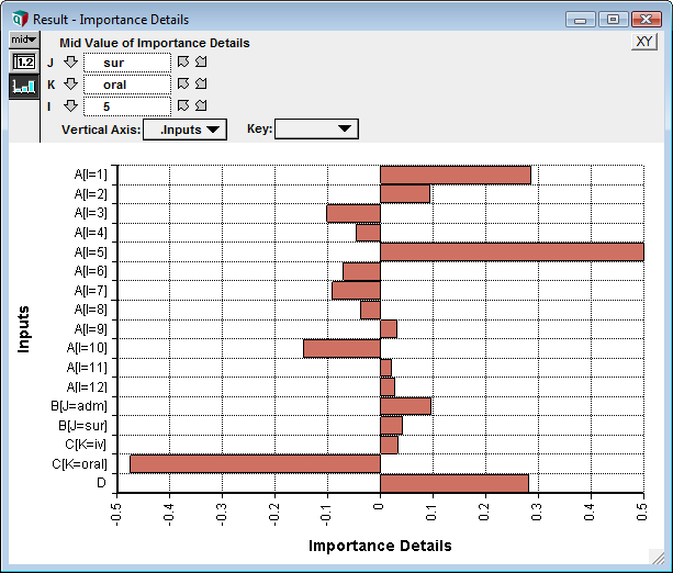
When the function is evaluated, it locates all chance variable ancestor nodes, and flattens their inputs into a single dimension, which becomes a local index named .Inputs. It collects the input samples for all inputs and performs the indicated analysis relative to the output, giving a sensitivity for every input cell. The following graph shows an example result for the above model:

Three slices appear at the top in this example. These slicers reflect the fact that the output in this example is three-dimensional, and these are the indexes of the output. Each out cell has its own sensitivity graph -- here we're seeing the sensitivity of inputs to the output:Result1[J = "sur", K = "oral", I = 5]

Every input cell appears in this result. Typically the total number of input "cells" will be overwhelming. When this isn't the case (as in this simple example with only 17 cells), a single details node may be all you need.

When you show the result the first time, access the graph setup dialog and check "Swap XY" to obtain horizontal bars, and then put the .Inputs index on the vertical axis.

Input Number

Here we limit the number of inputs to a given number. The Input_number node is defined as

SensitivityIndex(Importance_details, 5)

The second parameter is the maximum number of inputs to show. This variable becomes an index. It is preferable to use a variable node, rather than an index node, so that the value is not evaluated immediately when the model is loaded.

Input Descriptor

This variable is defined as:

InputDescriptors(Importance_details, Input_number)

The parameters are the identifiers for the two variables already created. This function assembles the names for the input cells that will be retained. The result is an array having the Input_number dimension, as well as any dimensions of the Result variable.

If you prefer the bars to be sorted by size in the final graph, you can embellish the definition of Input_descriptor as follows:

IntToString(Input_number, 3) & ". " & InputDescriptors(Importance_details, Input_number)

This embellishment numbers each input in such a way so that when the graphing engine sorts the labels, the bars will be ordered by size.

Importance_graph

This final node is the final importance graph of interest. If you have not used the embellishment mentioned for Input_descriptor, it is sufficient to define this as:

ImportanceGraph(Importance_details, Input_descriptor)

If you have used the embellishment, then use the following:

ImportanceGraph(Importance_details, InputDescriptors(Importance_details, Input_number))

To get the desired graph, the result graph itself must be twiddled some. To do this, show the result, and press the XY button on the top right of the graph window. This brings up the XY Comparison Sources dialog. Check Use another variable and add the Input_descriptor variable to the list, then press OK.

Next, in the Graph setup dialog, check Swap XY. And finally, pivot the graph so that Input Descriptor is used as the Vertical Axis and Input Number is used as the common index. To start, set the Key to Nothing, although one you get accustomed to the result, some informative graphs can result by selecting an index as the key. We have our final importance graph.

The following shows the final Importance_graph when using the embellishment for ordering the bars, and when showing the top 10 inputs.