Array Abstraction
(in-progress)
Array abstraction is one of the most powerful features in Analytica. Although conceptually simple, Analytica modelers find that their mastery of array abstraction continues to improve over the course of years. Array abstraction provides many benefits:
- Flexibility: Easy to alter an index, e.g., adding or deleting elements.
- Hyper-flexibility: Easy to adjust the dimensionality of a model, even late in the modeling process.
- Direct what-if analysis and parametric analysis.
- Simplifies expressions, which increases transparency
- Reduces the cognitive load of the modeler, with dramatic productivity gains during model creation.
- Speed - Analytica is an array-based semi-interpreted language, but array operations, the bulk of the computation, occur in "native code".
- Representational Power: Any simple scalar function becomes a powerful array function when abstracted.
- Synergy with probabilistic inference: Monte Carlo and Latin hypercube simulation are accomplished in Analytica through array abstraction. The Run index (i.e., the simulation index), is just another dimension, and the propagation of uncertainties through the model is an instance of array abstraction at work.
Array abstraction of a scalar function
One parameter function
The function Sqrt(x) computes the square root of «x». When you supply an array as a parameter, array abstraction iterates the function over all elements of the array and returns an array with the same dimensionality as the original.
- A :=
 Sqrt(A) :=
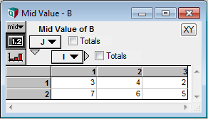


Sqrt is an example of a scalar function with one parameter. We say that it treats its parameter as atomic, or it treats its parameter as an atom.
Parameters have same indexes
The plus operator treats both its parameters as atoms. If both values supplied to the parameters have the same dimensionality, then array abstraction iterates over each index combination, producing an array result with the same dimensionality as the parameters.
- Variable B :=
Sqrt(A)
- A + B →


An array parameter with a scalar parameter
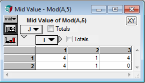
The Mod(x,y) function returns the remainder of dividing «x» by «y». It treats both parameters as atoms. When one parameter is an array and the other is scalar, array abstraction iterates over each cell of the array and applies the function using the same scalar value.
- Mod(A,5) →

Equivalence of a scalar and a non-varying array
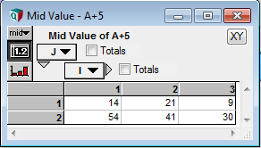
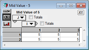
When you combine an array with a scalar, you get the same result as you would get if you combined the array with another array having the same indexes, but where every cell contains the scalar value.
- + 5 →
- +
 →
→


We say that an array that does not vary is equivalent to scalar with respect to array abstraction. It is a general principle that exchanging a value with an equivalent value in a computation produces an equivalent result. The indexes of the new result might be different, but if so, the result will be constant along any index that does not appear in its equivalent result.
This principle of equivalence gives rise to a general principle in Analytica modeling: You only need to include an index if the data you are representing varies over that index.
An inverse perspective is that you can conceptualize any value has if it has every index, but does not vary along those indexes that aren't shown.
Enable comment auto-refresher