Kernel Density Smoothing
Density Estimation Methods
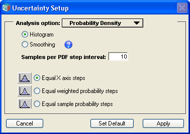
Histogram options 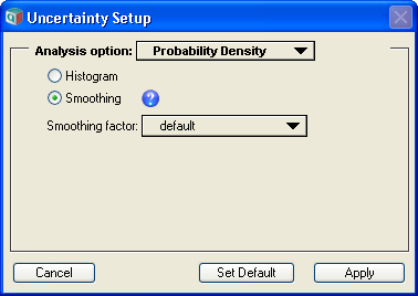
Kernel Density Smoothing options


Analytica represents the uncertainty of a variable as a Monte Carlo sample of representative points. The various uncertainty result views, including the Probability Density view, are all derived from the underlying sample when the result window is shown. Analytica has two basic methods for obtaining the estimate of the probability density from the underlying sample: Histogramming and Kernel Density Smoothing. The method to be used can be selected via the Uncertainty Options dialog as seen in the images above. The smoothing method is new to Analytica 4.4.

PDF result via Histogramming 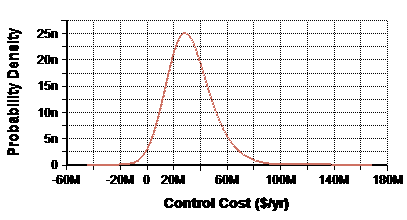
PDF result via Kernel density estimation


Histograms
The histogram method divides the range of possible values into distinct non-overlapping bins, then counts how many samples land in each bin. The center value for each bin is then plotted, with the density estimate equal to the fraction of points that landed in that bin divided by the width of the bin.
There are two basic ways to divide the range of possible values into bins: Equal-X or Equal-P.
The Equal-X method divides the range from the smallest to largest occurring value into equal sized bins. The number of points landing in each bin may vary considerably from bin to bin, and some bins may have no points in them at all.
The Equal-P method divides the cumulative probability axis (from 0.0 to 1.0) into equal sized intervals, causing the bins to be sized so that an approximately equal number of points land in each bin. The width of each bin varies.
In normal Monte Carlo sampling, every sample point is weighted equally. Some techniques such as rare-event modeling, importance sampling, and Bayesian likelihood posterior computations make use of non-equally weighted sampling. When these techniques are employed, two methodologies for Equal-P sampling are possible: Equal weighted steps and Equal sample steps. With equally weighted probability steps, bins are sized so that each bin ends up with approximately the same total probability weight. With equal sample steps, bins are sized so that a nearly equal number of points land in each bin. In the latter case, the weight of points may vary substantially from bin to bin (in fact, some bins may end up with zero weight when points with zero weight exist).
When using the histogram method, you have control over the average number of samples per bin. This parameter controls both how smooth the resulting PDF estimate is, and how many points are plotted. As you increase sample size, you will often want to increase this value as well, since with more sample points you are able to attain a smoother meaningful curve. Often a value approximately equal to [math]\displaystyle{ \sqrt{sampleSize} }[/math] produces pretty good results.
The PDF result for a histogrammed PDF uses the Step-line style by default, to emphasize the bins involved. From Graph setup dialog you can change this to a normal line style for a different (smoother) effect.
Kernel Density Smoothing
Kernel Density Smoothing, also known as Kernel Density Estimation (KDE), replaces each sample point with a Gaussian-shaped Kernel, then obtains the resulting estimate for the density by adding up these Gaussians.
To apply this method, a bandwidth, w, for each Gaussian Kernel must be selected -- a larger bandwidth results in greater averaging and hence smoother curves, but may also artificially increase the apparent variance in your overall uncertainty.
Mathematically, the estimated probability density at x is computed as:
- [math]\displaystyle{ f(x) = \sum w_i K_w(x-s_i) }[/math]
where [math]\displaystyle{ s_i }[/math] are the values in the Monte Carlo sample, [math]\displaystyle{ K_w(x) }[/math] is the zero-centered kernel function with bandwidth w, and [math]\displaystyle{ w_i }[/math] is the weighting of each point with [math]\displaystyle{ \sum w_i = 1 }[/math]. With standard unweighted Monte Carlo, [math]\displaystyle{ w_i = 1/sampleSize }[/math]. The Gaussian Kernel that is used is given by:
- [math]\displaystyle{ K_w(x-s_i) = {1\over{\sqrt{2\pi}w}} e^{-{1\over 2}\left({{x-s_i}\over w}\right)^2} }[/math]
In general, the selection of an appropriate bandwidth is difficult. A good choice depends on the data itself, the nature of the distribution, and the sample size. Analytica analyzes the data to derive what it deems to be the "optimal" bandwidth for the data set, and uses this value when the default smoothing factor is selected. The actual bandwidth used adapts to variations in data and to changes in sample size in a consistent manner. If you wish to average even further, or if you wish to view more detail, you can adjust the smoothing factor.
An Example
To understand how Kernel Density Smoothing works, consider this simple example. We have 10 points sampled from an underlying distribution, and in this example we will use a bandwidth of 0.4. First, we replace each point with a Gaussian with a width of 0.4, centered on the data point. Then we sum these to obtain the total estimate:

Each sample point is replaced by a Gaussian Kernel (red curves), then they are summed (blue).

Number of points plotted
With probability density smoothing, the smoothness and the number of points plotted are independent (unlike the histogram view, where increasing samples per bin reduces noise and reduces the number of points (bars). The Uncertainty Setup dialog lets you control the smoothness factor, but not over the number of points plotted. It usually plots 1000 points, which you can see by switching the view from graph to Table, where the .Step index has 1000 elements.
The smoothing uses the Fast Gaussian Transform letting it plot so many points almost instantaneously. For extremely large sample sizes, the smoothing method displays the density function much faster than the histogram method.
In rare situations, you may wish to control the number of points plotted. You can do this using by creating another variable that uses the Pdf function,which lets you set the number of points as a parameter.
Degree of Smoothing
Analytica analyzes the underlying sampling data and the sample size to arrive at a suggested degree of smoothing (the optimal bandwidth). You can, however, override this to obtain greater detail or greater smoothness as you see appropriate for particular cases. The smoothness factor gives you these options:
- maximum detail: minimum h value
- medium detail: medium low h value
- default: system determined h value
- medium smoothing: medium high h value
- maximum smoothing: maximum h value
As the bandwidth h decreases, the KDE smoothed PDF gets more sensitive to the random variation in your random sample, and can get quite wavy. As bandwidth h increases, the KDE smoothed PDF gets less sensitive to random variation and gets lots smoother, however, the match to the true underlying PDF may not be so good. Greater degrees of smoothing will artificially increase the apparent variance of KDE curve and lower the peak.
Determining the optimal bandwidth, h, value is a difficult problem in general. The smoothing factor is offered as a way to try different h values, and judge, by eyeballing the graphs produced, what looks best.
One clue here: compare the KDE smoothed graph with the histogram, to determine what smoothing factor seems to smooth the original histogram best. Also, in this process, for the histogram, try different "Samples per PDF step interval" values, since the histogram's random variation is sensitive to this. Find the best fit, between combinations of the smoothing factor and the samples per PDF step interval, and that might well be your best estimate of the underlying PDF.
Downsides of Smoothing
Smoothing has the effect of increasing the apparent variance in your uncertainty. Greater amounts of smoothing cause the uncertainty to appear larger than it may actually be. This effect also has the effect of lowering the height of your peaks.
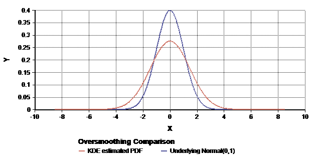
Large smoothness factors can increase the apparent variance.
Here the true underlyingNormal(0, 1)distribution is shown in blue, with the estimated PDF using a large smoothing factor is shown in red.

When a given mode of your underlying distribution has a variance of [math]\displaystyle{ \sigma^2 }[/math] and a bandwidth of [math]\displaystyle{ w }[/math] is used for smoothing, the effective plot can be expected to portray a variance of about [math]\displaystyle{ \sigma^2+w^2 }[/math]. The impact on the effective standard deviation in the displayed plot can be visualized as a right-triangle, where the underlying standard deviation and the bandwidth are the sides, and the effective plotted standard deviation is the hypotenuse.
The triangle visualization makes it fairly clear that the distortion from smoothing is small when [math]\displaystyle{ w \ll \sigma }[/math]. But when the smoothing reaches comparable levels, the distortion can be substantial. You should visualize this triangle analogy for each mode of your distribution.
The default bandwidth selected by Analytica (and any of the "more detailed" options) strikes a reasonable balance between smooth resulting plots and this distortion. But it is worth being aware of it. Histogramming is not subject to this same distortion.
A second distortion from smoothing is the "rounding" of rapid cut-offs. For example, a Uniform(0, 1) distribution would ideally be plotted with vertical edges. Smoothing, however, rounds the edges and gives the appearance of tails.
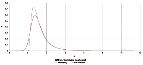
Smoothing may also give the impression of tails extending slightly into the negative region for positive-only uncertain variables, especially when the initial "rise" in the underlying density is very steep.
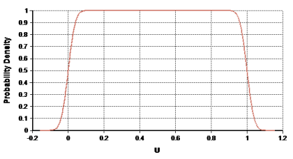
Smoothing can cause artificial rounding of sharp edges.
Here aUniform(0, 1)distribution is shown.Smoothing can extend tails into the negative region.
Here aLogNormal(1, 2)distribution is shown.


History
Introduced in Analytica 4.4.
Enable comment auto-refresher