Example 3: Beer Distribution with Limited Routes

Analytica Optimizer GuideOptimizing with ArraysExample 3: Beer Distribution with Limited Routes

The restriction of possible routes can be cumbersome in some optimizing environments. As this example will show, in Analytica, it is a simple matter of changing the dimension of the decision array.

Model Description

In the previous examples, we allowed all five Breweries to ship to all four Markets, presenting 20 possible routes. In this example, we confine the shipments to 10 chosen routes and disallow the rest.

Setting Up the Model

To explore and follow this example in Analytica, run the Beer Distribution LP 3.ana model in the Optimizer Examples folder.

In this section, we start with the model from Example 2, detailing changes only.

Create a Route Index

First, we create an index of approved routes. These are specific combinations of Brewery and Market.

Index Route := 
     ['Fairfield North', 'Fairfield South', 'Fairfield West',
     'Fort Collins North', 'Fort Collins South',
     'Jacksonvile East',
     'Merrimack North', 'Merrimack East',
     'St Louis North', 'St Louis East']

Redefine the Decision input array

In previous examples, we defined the Decision input as a two-dimensional array. In this example we redefine it to be a one-dimensional array along the index of approved routes. Once again, we can insert a dummy value of 1 for the non-optimized quantities since they are not used anywhere else in the model.

Edit the Intrinsic Indexes list

Make sure to also edit the Intrinsic Indexes list. Remove Brewery and Market, and add Route to the list.

Variable Shipment_Quantity := Array(Route, 1)
Shipment_Quantity attribute Intrinsic Indexes := [Route]

Redefine the Objective and its inputs

The Objective representing Total Distribution Cost should now sum over the Route index instead of Brewery and Market.

Objective Total_Dist_Cost := Sum(Shipment_Quantity*Dist_per_case, Route)

All inputs to Total Distribution Cost should be also dimensioned by Route. We redefine the Distance array using corresponding values from the original table.

Variable Distance :=
     Table(Route)(1.8, 2.2, 0.1, 0.3, 1.2, 0.6, 1.2, 0.2, 0.5, 0.8)

Original Distance Array:

Redefined Distance Array:

Creating Index Maps

Constraint arrays do not change indexes in the new model. Production Limits still apply to Breweries, and Delivery Targets still apply to Markets. But the Shipment Quantities array no longer contains these indexes. To solve this dilemma, we start by making index maps relating the Route index to Brewery and Market. An index map is a one-dimensional array that associates a coarse index with a fine index. The map uses the fine index as its dimension and lists corresponding elements of the coarse index.

Create a new variable titled Route / Brewery map.

Variable Route_Brewery_map := Table(Route)
     ('Fairfield', 'Fairfield', 'Fairfield',
     'Fort Collins', 'Fort Collins',
     'Jacksonville',
     'Merrimack', 'Merrimack',
     'St Louis', 'St Louis' )

Create a new variable titled Route / Market map.

Variable Route_Market_map :=Table(Route)
     ('North','South','West','North','South',
      'East','North','East','North','East')

Using Aggregate()

The Aggregate function can use these maps to create aggregated sums. This allows us to convert Shipment Quantities from the fine index (Route) to the coarse target indexes (Brewery or Market).

The basic syntax of the AggregateFunction is:

Aggregate(input_array, map, fine_index, target_index)

Aggregate Shipment Quantities

Now we can create suitable inputs for the Constraint nodes.

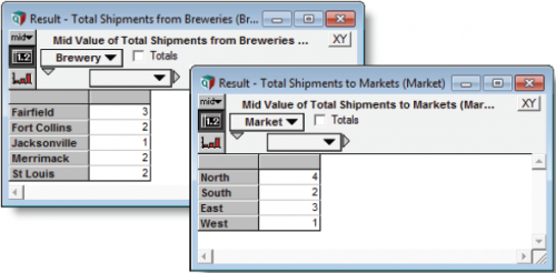
Create a new variable titled Total Shipments from Breweries

Variable Ship_from_Brewery := 
     Aggregate(Shipment_Quantity, Route_Brewery_map, Route, Brewery)

Create a new variable titled Total Shipments to Markets

Variable Ship_to_Market := 
     Aggregate(Shipment_Quantity, Route_Market_map, Route, Market)

You can evaluate the aggregated arrays to verify that they represent Shipment Quantities aggregated by Brewery and Market. Input Quantities are 1 for each Route, so these aggregated sums represent the number of routes associated with each Brewery or Market.

Edit Constraint Inputs

Edit the Supply Constraint to use Total Shipments from Breweries as an input. Brewery is still an intrinsic index for this node.

Constraint Supply_Constraint := Ship_from_brewery <= Production_Limits
Supply Constraint attribute Intrinsic Indexes := [Brewery]

Edit the Demand Constraint to use Total Shipments to Markets as an input. Market is still an intrinsic index for this node.

Constraint Demand_Constraint := Ship_to_market >= Delivery_Target
Demand Constraint attribute Intrinsic Indexes := [Market]

Checking the Result

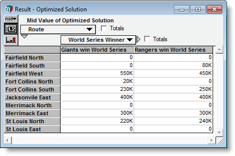
Evaluate the Optimized Solution array to see the result for the limited route example. This is now a two-dimensional array indexed by the intrinsic Route index and the extrinsic World Series Winner index.

Example 3: Beer Distribution with Limited Routes

Contents

Model Description

Setting Up the Model

Checking the Result

See Also