Tutorial: Dynamic system model
This chapter shows you how to:
- Use the Dynamic() function and the system variable Time
- Customize the appearance of variable nodes
- Organize a model using modules
- Make duplicates of nodes and modules
- Create aliases of variable nodes
- View the results of two variables simultaneously
Before starting this chapter you should know how to perform the following actions which will no longer be described in detail:
Create a new model; Open an existing model; Save; Save As... (See Using the Rent vs. Buy Model)
Create and define new variables; Enter attributes in Attribute or Object windows; Draw influence arrows between nodes. (See Creating Models)
You should also be familiar with Array variables and Index variables. (See Working with Arrays (Tables))
Using the Time index
In this model you will set up a dynamic system to model a predator/prey relationship. The populations of foxes and hares will be set up as state variables: one-dimensional arrays indexed by Time.
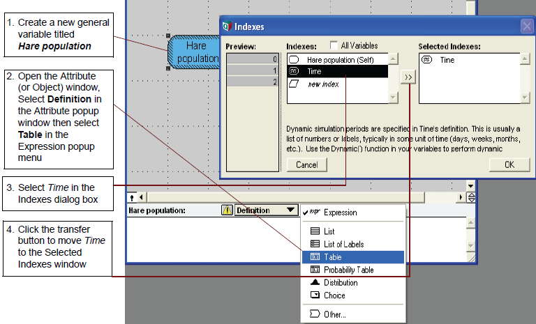
Start by opening a new model and titling it Foxes and Hares Tutorial. Create a general variable titled Hare population.
Using either the Attribute window or the Object window, place the cursor in the definition field and choose Table from the expression popup menu. The Indexes window will appear.
Notice that Time is listed as one of the indexes in the left hand window. You did not have to define this index before using it. Time is a system index in Analytica that is always available to you. Note that it is distinguished by the system variable icon (![]() ). Although it is a system variable, the values of Time can be edited just like any other index.
). Although it is a system variable, the values of Time can be edited just like any other index.
Select the Time index and click the transfer button (![]() ) to select it as an active index in the right-hand window. Click OK to exit the Indexes window.
) to select it as an active index in the right-hand window. Click OK to exit the Indexes window.
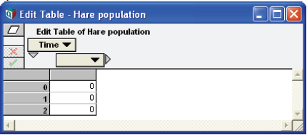
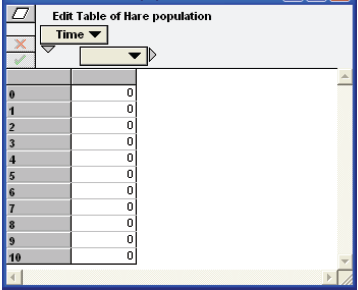
Analytica will show an edit table for the Hare population variable. Notice that the default index values for Time are 0,1, and 2. You will need to have more than just three time points in your dynamic simulation.
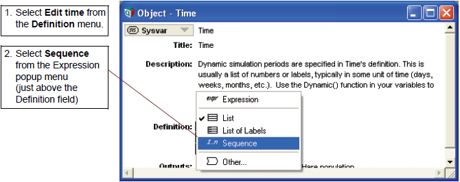
Go to the Definition menu and select Edit time. Click the Expression popup menu and select Sequence. Analytica will prompt to make sure you want to change the Time index to a Sequence. Click OK.
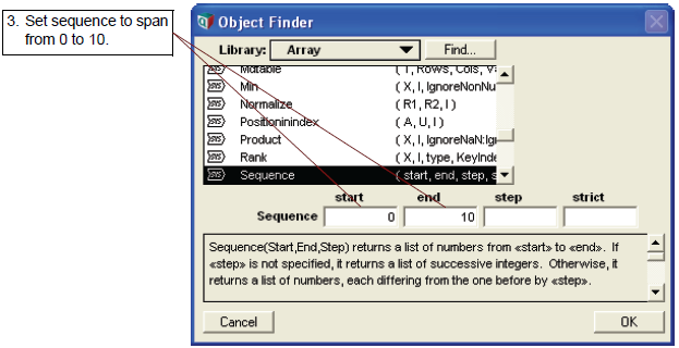
Edit the sequence by keeping 0 for the start value and entering 10 for the end value. Click OK to exit the Object finder window.
If the edit table for Hare population is not already open select the Hare population node and click on the Result button ([[![]() ]]). Notice that our time index now goes from 0 to 10. We will leave the values of the Hare population zero the moment.
]]). Notice that our time index now goes from 0 to 10. We will leave the values of the Hare population zero the moment.
Setting up the Hare sub-model
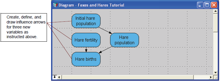
Create three new general variables titled Initial hare population, Hare fertility, and Hare births. Draw influence arrows as follows:
- from Hare fertility to Hare births
- from Initial hare population to Hare population
- from Hare population to Hare births
Define Initial hare population as 500. Change its Identifier to Hare_zero.
Define Hare fertility as 60%. We will take this to mean that the number of newborn hares will be equal to 60% of the total population during the previous time period!
Define Hare births as Hare_population * Hare_fertility. This is the total number of births during a time period.
Using the Dynamic() function
Now we consider how the hare population will develop over time. The hare population will be influenced by the number of hare births, which will be influenced by the hare population during the previous period. Ultimately the value of Hare population depends on the value of itself during the previous time period. We can address this situation using the Dynamic() function.
Using either the Attribute window or the Object window, open the Definition field of the Hare pop- ulation variable. Click on the Expression popup menu and select ![]() .
.
Delete the existing table expression and replace it with the following:
The Dynamic() function can be entered directly as an expression or accessed as a built-in func- tion (by selecting Other... in the expression popup menu). It is listed under the Special library heading.
Note that the Dynamic() function automatically incorporates the Time system variable. It was not necessary to initially define our variable as a table indexed by Time, although this step was included in the first section of this chapter to illustrate the Time index.
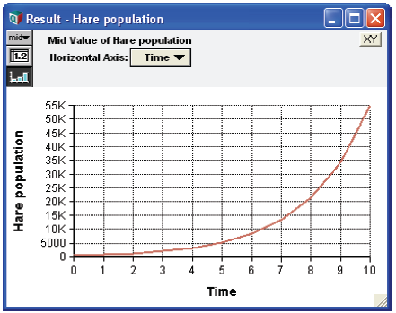
Select the Hare population node and click the Result button (![]() ).
).
This is a simple exponential growth curve. It represents a rapidly multiplying population of immortal hares with no natural predators and an unlimited food supply. You will need to introduce a limiting factor to avoid this buried-in-bunnies scenario.
Completing the Hare sub-model
Quickly before it’s too late, create four new general variables as follows:
Finally you need to change the definition of Hare population as follows:
Dynamic(hare_zero, self[time -1] + hare_births[time - 1]- hare_deaths[time - 1])
See Also
| Creating the Party Problem Model <- | Creating the Foxes and Hares Model | -> Sharing Models with Others |


Enable comment auto-refresher