Parametric discrete distributions
Bernoulli(p)
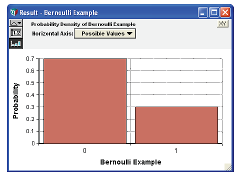
Defines a discrete probability distribution with probability «p» of result 1 and probability (1 - «p») of result 0. It generates a sample containing 0s and 1s, with the proportion of 1s is approximately «p». «p» is a probability between 0 and 1, inclusive, or an array of such probabilities. The Bernoulli distribution is equivalent to:
If Uniform(0, 1) < P Then 1 Else 0
Library: Distribution
Example: The domain, List of numbers, is [0, 1].
Bernoulli_ex := Bernoulli (0.3) →
See also Bernoulli().
Binomial(n, p)
An event that can be true or false in each trial, such as a coin coming down heads or tails on each toss, with probability «p» has a Bernoulli distribution. A binomial distribution describes the number of times an event is true, e.g., the coin is heads in «n» independent trials or tosses where the event occurs with probability «p» on each trial.
The relationship between the Bernoulli and binomial distributions means that an equivalent, if less efficient, way to define a Binomial distribution function would be:
Function Binomial2(n, p)Parameters: (n: Atom; p)Definition: Index i := 1 .. n;
The parameter «n» is qualified as an Atom to ensure that the sequence 1.. n is a valid one-dimensional index value. It allows Binomial2 to array abstract if its parameters «n» or «p» are arrays.
See also Binomial().
Poisson(m)
A Poisson process generates random independent events with a uniform distribution over time and a mean of m events per unit time. Poisson(m) generates the distribution of the number of events that occur in one unit of time. You might use the Poisson distribution to model the number of sales per month of a low-volume product, or the number of airplane crashes per year.
Geometric(p)
The geometric distribution describes the number of independent Bernoulli trials until the first successful outcome occurs, for example, the number of coin tosses until the first heads. The parameter «p» is the probability of success on any given trial. See also Geometric().
HyperGeometric(s, m, n)
The hypergeometric distribution describes the number of times an event occurs in a fixed number of trials without replacement, e.g., the number of red balls in a sample of «s» balls drawn without replacement from an urn containing «n» balls of which «m» are red. Thus, the parameters are:
- «s» - The sample size, e.g., the number of balls drawn from an urn without replacement. Cannot be larger than «n».
- «m» - The total number of successful events in the population, e.g, the number of red balls in the urn.
- «n» - The population size, e.g., the total number of balls in the urn, red and non-red.
See also HyperGeometric().
NegativeBinomial(r, p)
The negative binomial distribution describes the number of successes that occur before «r» failures occur, where each independent Bernoulli trial has a probability «p» of being a success. The domain is the set of non-negative integers. The Geometric distribution is a special case when «r»=1. When «r»>1 the distribution tends to be bell shaped.
There are three common bell-shaped discrete distribution types on the integers 0, 1, 2, ..., namely the binomial, Poisson and the negative binomial. A binomial has a variance that is less than the mean, a Poisson has a variance equal to the mean, and a negative binomial has a variance greater than the mean.
See also NegativeBinomial().
Uniform(min, max, integer: True)
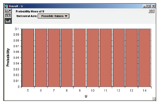
The Uniform distribution with the optional «integer» parameter set to True returns discrete distribution over the integers with all integers between and including «min» and «max» having equal probability.
Uniform(5, 14, Integer: True) →
See also Uniform().
Wilcoxon(m, n, exact)
The Wilcoxon distribution characterizes the distribution of the Wilcoxon rank-sum statistic, known as the U-statistic, that is obtained when comparing two populations with unpaired samples having sizes «m» and «n». The rank-sum test is a non-parametric alternative to the Student-t test, which unlike the Student-t test, does not assume that the distribution is normally distributed. The distribution is non-negative and discrete, and approaches a normal distribution for large «m» + «n».
Given two samples, x of size m and y of size n, the U-statistic is the number of pairs (xi, yj) in which xi < yj.
Like other distribution functions in Analytica, the Wilcoxon(m, n) function generates a random sample, which in this case would be the distribution of U-statistic values when two sampes of size «m» and «n» and equal distributions are compared. Also available as built-in functions are ProbWilcoxon(u, m, n), CumWilcoxon(u, m, n) and CumWilcoxonInv(p, m, n), the analytic probability distribution, cumulative probability and inverse cumulative probability functions respectively. If you want to perform a rank-signed test, the CumWilcoxon(u, m, n) function is the one to use, since it returns the p-value. Although they are built-in functions, the analytic functions aren’t listed on the Definition menu libraries until you add the Distribution Densities library to your model.
The exact parameter controls whether an exact algorithm is used or a Normal approximation. By default, a Normal approximation is used when «m» + «n» >100, which has been observed empirically to be within 0.1% accuracy. Time and memory usage can be get excessive when «m» + «n» gets large. When accuracy requirements are not demanding, efficiency can be gained by using Wilcoxon(m, n, exact: m + n < 50), or CumWilcoxon(m, n, exact: m + n < 50), etc.
See Also


Enable comment auto-refresher