UncertainLMH distribution
New in Analytica 5.0
UncertainLMH( xLow, xMedian, xHigh, pLow, lb, ub)
Specifies a smooth continuous distribution from «xLow», «xMedian» and «xHigh» estimates. By default these are the 10-50-90 percentile estimates. You can specify the optional «pLow» percentile level as a positive number less than 0.5 to use different percentile levels. For example, setting «p» to 0.25 treats «xLow»-«xMedian»-«xHigh» as 25-50-75 percentile estimates.
When «lb» (lower bound) and «ub» (upper bound) are not specified, the distribution is unbounded (tails in both directions). When «lb» is specified, it becomes a lower-bound, and when «ub» is specified it becomes an upper bound. Hence, this distribution function can be used to specify unbounded, semi-bounded and fully-bounded smooth continuous distributions.
The distribution return is called a Keelin MetaLog SPT distribution" (Symmetric Percentile Triplet), or a Keelin distribution. This distribution was introduced in
- Thomas W. Keelin (Nov. 2016), "[bsonline.informs.org/doi/10.1287/deca.2016.0338 The Metalog Distribution]", Decision Analytics, 13(4):243-277,
The distribution used by this function is a 3-term Keelin MetaLog.
Feasibility
It is required that the parameters specified are ordered as «lb» < «xLow» < «xMedian» < «xHigh» < «ub». However, not all ordered combinations of percentile estimates result in a valid 3-term Keelin distribution. Those combinations that are valid are called feasible, and parameter combinations that cannot be fit exactly are called infeasible. Infeasible combinations are typically very extreme. When an infeasible combination of parameters is encountered, the error message identifies the range of possible values for «xMedian» that would result in a feasible distribution given the other parameters.
Examples
An unbounded smooth continuous distribution with a 10% probability of being <= 8, a 50% probability of being <= 29, and a 90% probability of being less that 44. In other words, the 10-50-90 estimates are 8,29,44:
UncertainLMH(8, 29, 44)→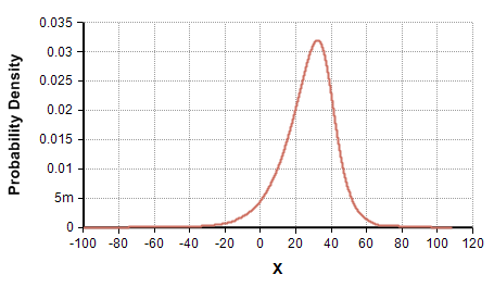
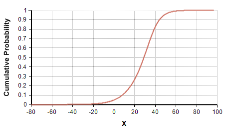


A positive-only (semi-bounded) distribution with 10-50-90 percentiles of 8, 29 and 44:
UncertainLMH(8, 29, 44, lb:0)→
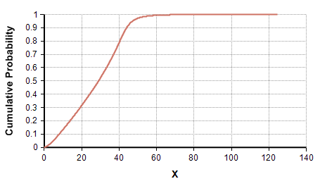


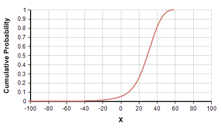
A semi-bounded from above distribution with 10-50-90 percentiles of 8, 29, 44 and an upper bound of 60
UncertainLMH(8, 29, 44, ub:60)→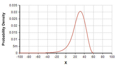


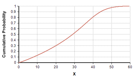
A full bounded (between 0 and 60) distribution with 10-50-90 percentiles of 8, 29 and 44.
UncertainLMH(8, 29, 44, lb:0 ub:60)→


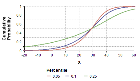
Comparison of three unbounded distributions with different percentile levels. 5-50-95, 10-50-90 and 25-50-75. Notice that the CDF's value at X=8 is equal to the percentile level, that all three CDF curves pass through (29, 0.5), and that the CDF at x=44 is 1 minus the percentile level.
Index percentile := [5%, 10%, 25%] Do UncertainLMH(8, 29, 44, percentile)→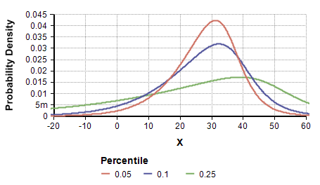


Enable comment auto-refresher