Normal distribution

Normal(mean, stddev, over)

Creates a normal or Gaussian probability distribution with «mean» and standard deviation «stddev». The standard deviation must be 0 or greater. The range [mean - stddev, mean + stddev] encloses about 68% of the probability.

As with all distribution functions in Analytica, Normal allows you to specify an optional parameter «over». Without this parameter, with scalar «mean» and «stddev» parameters, a single random normal variate is generated. If you want the random variate to vary independently across one or more indexes, then those indexes can be specified in «over». If the «mean» or «stddev» parameters are array-valued, then Normal returns an array of random values that are statistically independent across the indexes of the parameters.

When to use

Use a normal distribution if the uncertain quantity is unimodal and symmetric and the upper and lower bounds are unknown, possibly very large or very small (unbounded). This distribution is particularly appropriate if you believe that the uncertain quantity is the sum or average of a large number of independent, random quantities.

Library

Distributions

Parameter Estimation

Suppose you want to fit a Normal distribution to historical data. Assume your data is in an array, x indexed by I. The parameters of the Normal distribution as obtained using:

«mean» := Mean(x, I)

«stddev» := SDeviation(x, I)

Theoretical Properties

In this section, we'll use symbols [math]\displaystyle{ \mu }[/math] and [math]\displaystyle{ \sigma }[/math] to denote the «mean» and «stddev» values.

Density Function: The density at a point x is returned by the expression Dens_Normal(x, mean, stddev), from the Distribution Densities library, which is given by [math]\displaystyle{ \frac{1}{\sqrt{2\pi\sigma^2}}\,e^{ -\frac{(x-\mu)^2}{2\sigma^2} } }[/math]

Cumulative Probability: The probability that the value is less than or equal to x is returned by the expression CumNormal(x, mean, stddev), and is given by [math]\displaystyle{ \frac12\left[1 + \mbox{erf}\left( \frac{x-\mu}{\sqrt{2\sigma^2}}\right)\right] }[/math]

Statistics

Mean = «mean» = [math]\displaystyle{ \mu }[/math]
Standard Deviation = «stddev» = [math]\displaystyle{ \sigma }[/math]
Variance = [math]\displaystyle{ «stddev»^2 = \sigma^2 }[/math]
Skewness = 0
Kurtosis = 0

Central Limit Theorem: The CLT states that under non-degenerate conditions, the sum of a large number of independent random variables is approximately normally distributed. This holds even when the individual random variables are not normally distributed, and requires just that their distributions have finite variance. This property makes Normal distributions highly ubiquitous in statistics and in nature. Most common distributions end up being approximated by normal distributions in certain extremes.

Approximations by Normal Distribution: These are examples of distributions that are approximated by the Normal distribution:

The Binomial(n, p) approaches Normal(n*p, n*p*(1 - p)) when n is large.
The Poisson(mean) distribution approaches Normal(mean, Sqrt(mean)) as mean gets large.
The ChiSquared(dof) distribution approaches Normal(dof, Sqrt(2*dof)) as dof gets large.
The StudentT(dof) distribution approaches Normal(0, 1) when dof gets large.
The Wilcoxon and Mann-Whitney-Wilcoxon tests (for whether two distributions are equal in hypothesis testing) use the so-called Wilcoxon distribution(s), which is/are quickly approximated by a Normal distribution. See Binomial, Poisson, ChiSquared and StudentT.

Combination properties

When [math]\displaystyle{ X \sim Normal(\mu,\sigma) }[/math], then

[math]\displaystyle{ a*X+b \sim Normal\left(a*\mu+b, a*\sigma\right) }[/math]

When [math]\displaystyle{ X_1 \sim Normal(\mu_1,\sigma_1) }[/math] and [math]\displaystyle{ X_2 \sim Normal(\mu_2,\sigma_2) }[/math], then

[math]\displaystyle{ a*X_1+b*X_2 \sim Normal\left(a*\mu_1+b*\mu_2, \sqrt{a^2 \sigma_1^2 + b^2 \sigma_2^2} \right) }[/math]

When a Bayesian Prior is normally distributed as [math]\displaystyle{ Normal(\mu,\sigma) }[/math], the posterior after observing a random value, x, drawn from the distribution, is also normally distributed as is given by

[math]\displaystyle{ Normal\left({{\mu+x}\over 2}, {\sigma\over\sqrt{2}}\right) }[/math]

The Logarithm of a normally distributed variable obeys the LogNormal distribution.

The multivariate generalization of the Normal is the Gaussian distribution, parameterized by a mean vector an a Covariance matrix.

Examples

Normal(30, 5) →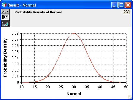

Brownian Motion

A discrete-time Brownian process in time can be encoded as:

Dynamic(0, Self[Time-1] + Normal(0, 1))

or as

Cumulate(Normal(0, 1, over: Time), Time )

Please take note of several subtleties with these examples. First, these two are not quite equivalent -- they treat the @Time = 1 case differently. Either can be adjusted to treat the first time point as fixed or random - this is left as an exercise for the reader (solution is in the discussion tab). Second, notice that the «over» parameter was necessary in the Cumulate example. Without it, the expression:

Cumulate(Normal(0, 1), Time)

would select a single delta value that would apply to all time periods, resulting in a straight line with a random slope, rather than a random walk. The «over» parameter is not required in the Dynamic example since the recurrence expression is re-evaluated at each time step, causing the random variates to be independent automatically.