Negative binomial distribution

(new to Analytica 4.5)

NegativeBinomial(r,p)

The negative binomial distribution is a discrete probability distribution that models the number of successes that occur before «r» failures, where each independent trial is a success with probability «p». The sample values are non-negative integers.

The NegativeBinomial distribution can be considered to be one of the three basic discrete distributions on the non-negative integers, with Poisson and Binomial being the other two. If we characterize discrete distributions according to the first two moments -- specifically how the variance compares to the mean -- then three distributions span the space of possibilities. For the Binomial distribution the variance is less than the mean, for the Poisson they are equal, and for the NegativeBinomial distribution the variance is greater than the mean. Turning this around, if you are trying to decide which of the discrete distributions to use to describe an uncertain quantity and all you have is the first two moments, then you can chose between these three distributions based on whether the variance is less than, equal to, or greater than the mean.

Probability Function

The probability distribution function for the NegativeBinomial is:

[math]\displaystyle{ P(x=k) = Combinations(k, k+r-1) * p^k * (1-p)^r }[/math]

The cumulative density is

[math]\displaystyle{ P(x\ge k) = 1-BetaI(p,k+1,r) }[/math]

Library

Distributions

Examples

A shoplifter has a 20% change of getting caught and convicted each time he commits the crime (hence, his probability of success is 80%). The third conviction carries jail time. The number of times he shoplifts and gets away with it before being thrown in jail is given by

NegativeBinomial(3,80%)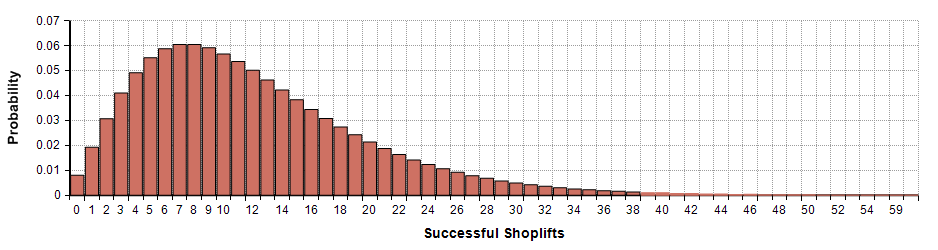

A certain baseball player hits a home run for every 12 times he is at bat. To beat Barry Bond's record of 73 home runs in a single season, the number of times he would need to be at bat would be given by

NegativeBinomial(74,1-1/12) + 74

In this case, when we talk about the NegativeBinomial distribution modeling the number of successes before a failure, here we apply this by calling a non-home run "a success", which happens with probability 1-1/12. To beat Barry Bond's record of 73, we need 74 home runs, and the since the total number of at bats includes both successes and failures, we add the 74 homeruns to the result. The cumulative distribution is shown in the next graph which shows that he has a 20% probability of beating the record if he can get to bat at least 800 times.

See Also

• CumNegativeBinomial(k,r,p)
• ProbNegativeBinomial(k,r,p)
• CumNegativeBinomInv(u,r,p)
• Binomial(n,p)
• Poisson(mean)
• BetaI, BetaIaInv, Combinations