Difference between revisions of "Making a Multi-D Scatter Plot"
(Setting up the data for the example) |
|||
| Line 15: | Line 15: | ||
Index Dim := [1,2,3,4] | Index Dim := [1,2,3,4] | ||
Index Dim2 := CopyIndex(Dim) | Index Dim2 := CopyIndex(Dim) | ||
| + | |||
| + | [[image:scatterExample2.jpg]] | ||
| + | |||
| + | 7. Define the covariance matrix. Create a variable named covar and set the definition type to Table. Select the Dim and Dim2 indexes and fill in the edit table with a covariance matrix: | ||
| + | |||
| + | [[image:scatterExample3.jpg]] | ||
| + | |||
| + | 8. Define the Gaussian distribution. Create a chance variable node named X and set the definition to: | ||
| + | Gaussian( 0, covar, Dim, Dim2 ) | ||
| + | |||
| + | [[image:scatterExample4.jpg]] | ||
| + | |||
| + | 9. Select Result-> Uncertainty Options... and set the sample size to 1000. (so we have more points on our plot) | ||
| + | |||
| + | [[image:scatterExample5.jpg]] | ||
| + | |||
| + | 10. Select X and show Result->Sample. Switch to graph mode if not already. | ||
| + | |||
| + | [[image:scatterExample6.jpg]] | ||
| + | |||
| + | 11. Switch to table view to examine the actual data. For convenience, pivot so that Index Dim forms the columns, Run the rows. | ||
| + | |||
| + | [[image:scatterExample7.jpg]] | ||
| + | |||
| + | == Setting the Coordinate Index = | ||
| + | |||
| + | At this point you have defined some data to graph, and are viewing the default graph. | ||
Revision as of 21:02, 6 February 2007
In this tutorial example, we'll plot the points from a 4-D Gaussian distribution as a scatter plot. You will learn how to set up a scatter plot when the coordinates of the data are organized as columns in a single table, and how such plots can be interactively pivoted to view the scatter points from each dimension.
First, let's create the data to be plotted. For this, we'll define a 4-D gaussian distribution. Follow these steps:
1. Start with a fresh model.
2. In the model's object window, fill in the title and description.
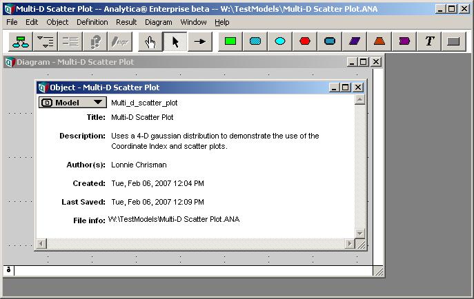
3. Close the object window.
4. Select File->Add Library... -> Multivariate Distributions.ana
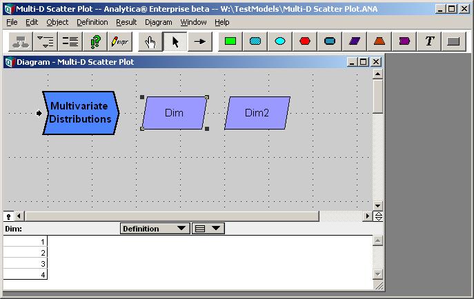
5. Create these two indexes:
Index Dim := [1,2,3,4]
Index Dim2 := CopyIndex(Dim)
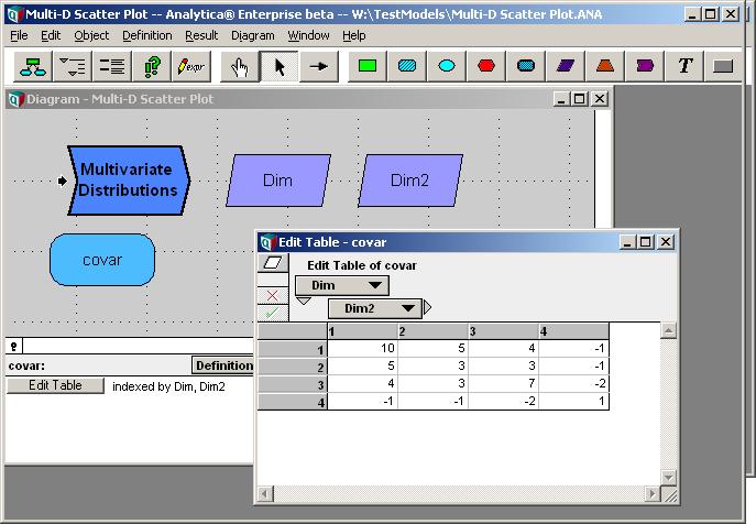
7. Define the covariance matrix. Create a variable named covar and set the definition type to Table. Select the Dim and Dim2 indexes and fill in the edit table with a covariance matrix:
8. Define the Gaussian distribution. Create a chance variable node named X and set the definition to:
Gaussian( 0, covar, Dim, Dim2 )
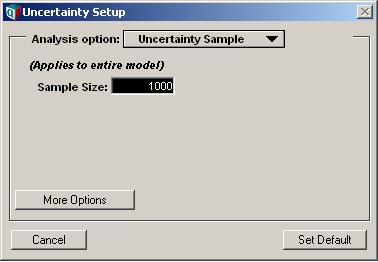
9. Select Result-> Uncertainty Options... and set the sample size to 1000. (so we have more points on our plot)
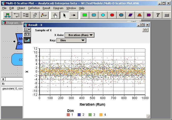
10. Select X and show Result->Sample. Switch to graph mode if not already.
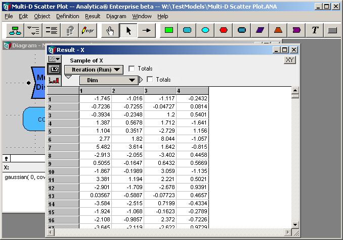
11. Switch to table view to examine the actual data. For convenience, pivot so that Index Dim forms the columns, Run the rows.
= Setting the Coordinate Index
At this point you have defined some data to graph, and are viewing the default graph.

Enable comment auto-refresher