Difference between revisions of "Mixture distribution"
(Created page with "A ''mixture distribution'', sometimes also called a ''mixture density'', is a distribution from the weighted combination of two or more component distributions. The component ...") |
(fixed a broken link) |
||
| (6 intermediate revisions by 2 users not shown) | |||
| Line 1: | Line 1: | ||
| − | A ''mixture distribution'', sometimes also called a ''mixture density'', is a distribution from the weighted combination of two or more component distributions. The component distributions can be univariate or multivariate. | + | [[Category:Concepts]] |
| + | |||
| + | __TOC__ | ||
| + | |||
| + | |||
| + | A ''mixture distribution'', sometimes also called a ''mixture density'', is a distribution formed from the weighted combination of two or more component distributions. The component distributions can be univariate or multivariate. | ||
{| border="0" | {| border="0" | ||
| Line 12: | Line 17: | ||
Suppose you have a population, where each individual in the population belongs to exactly one of several groups. If you can estimate the distribution of some quantity for each group, the distribution for the population as a whole is obtained as a mixture of these, with each component weighted as the fraction of the total population represented by that group. | Suppose you have a population, where each individual in the population belongs to exactly one of several groups. If you can estimate the distribution of some quantity for each group, the distribution for the population as a whole is obtained as a mixture of these, with each component weighted as the fraction of the total population represented by that group. | ||
| − | :Example: A highway is populated by | + | :Example: A highway is populated by 67% cars and 33% trucks. The weight of cars is distributed as <code>Normal(3200, 300)</code> pounds, whereas the weight of trucks is distributed as <code>Normal(12K, 4K)</code>. The variability distribution for all vehicles is a mixture of these, with the <code>Normal(3200, 300)</code> distribution given a weight of 0.67, the <code>Normal(12K, 4K)</code> given a weight of 0.33. |
| + | |||
| + | :{|border="0" | ||
| + | |[[image:Mixture_cars_truck.png|frame|Distribution of vehicle weights]] | ||
| + | |} | ||
| − | Another use arises when several situations are possible, but you don't know which situation you are in. If you have assessments for the uncertainty of a certain quantity for each situation, and you have an estimate for the probability of being in each situation, then the mixture of the | + | Another use arises when several situations are possible, but you don't know which situation you are in. If you have assessments for the uncertainty of a certain quantity for each situation, and you have an estimate for the probability of being in each situation, then the mixture of the distributions for each situation weighted by the probability gives your net uncertainty. |
| − | :Example: A stock trader knows that the FDA will soon be ruling on whether a certain company's new drug will be approved or not. He believes if it is approved, the companies stock price will see a change estimated at <code> | + | :Example: A stock trader knows that the FDA will soon be ruling on whether a certain company's new drug will be approved or not. He believes if it is approved, the companies stock price will see a change estimated at <code>Normal(180%, 40%)</code>, but if it is not approved he expects the price to change by <code>Normal(-60%, 30%)</code>. Since he believes there to be a 50% probability of approval, an equally weighted mixture can be used to model the projected change in stock price. |
| − | Mixtures are also used when [ | + | Mixtures are also used when [https://analytica.com/blog/combination-of-assessed-distributions| combining assessments from multiple experts]. The assessment distributions from each expert can be mixed using a subjective weight reflecting each expert's credibility. |
| − | The relative credibility of experts is not precisely-defined quantity, although it is can still be employed without too much confusion in practice. An alternate interpretation is that you can one expert is "correct" and the other experts are wrong. | + | :The relative credibility of experts is not a precisely-defined quantity, although it is can still be employed without too much confusion in practice. An alternate interpretation is that you can one expert is "correct" and the other experts are wrong. Strictly speaking, this does not make sense, since an assessment is a subjective representation of uncertainty, not something that has a "correct" or "incorrect" answer. However, using this idea, you can interpret the weighting to be the probability of each expert being the correct one. The mathematics of combination are the same, it is just a metaphor for interpreting the weights. |
When you are estimating uncertainty of a quantity, and you feel the uncertainty is bi-modal or multimodal, a mixture is usually the most direct and intuitive way to encode multimodal uncertainty. Most standard parametric distributions are unimodal (i.e., they have only one peak in the density graph), so you can't employ these alone. | When you are estimating uncertainty of a quantity, and you feel the uncertainty is bi-modal or multimodal, a mixture is usually the most direct and intuitive way to encode multimodal uncertainty. Most standard parametric distributions are unimodal (i.e., they have only one peak in the density graph), so you can't employ these alone. | ||
| + | |||
| + | == Difference between a mixture and a sum == | ||
| + | |||
| + | A mixture distribution is not the same as the distribution for the weighted [[sum]] of [[random]] variables. | ||
| + | |||
| + | :Example: There are 67 cars and 33 trucks on a road, with the weight of cars distributed as <code>Normal(3200, 300)</code> , and truck as <code>Normal(12K, 4K)</code>. The distribution of total weight is show here (compare this to the ''distribution of vehicle weights'' above): | ||
| + | |||
| + | :{|border="0" | ||
| + | |[[image:Mixtures_total_weight.png|frame|Uncertainty in the total weight of cars and trucks]] | ||
| + | |} | ||
| + | |||
| + | This is not a mixture at all. In fact, it is a [[Normal]] distribution, and is quite distinct visually. | ||
| + | |||
| + | == Encoding mixtures in Monte Carlo == | ||
| + | |||
| + | In the most common case, you will encode the uncertainty in your chance variables and let Monte Carlo propagate the uncertainty for you. A mixture is NOT formed as the weighted sum of distribution functions. That would be encoding the distribution of the weighted sum (e.g., the total weight of cars and trucks). | ||
| + | |||
| + | A two component mixture is usually encoded using and [[If|IF-THEN-ELSE]] with a [[Bernoulli]] for the [[If]] clause, as in this example: | ||
| + | |||
| + | :<code>If [[Bernoulli]](0.67) Then [[Normal]](3200, 300) Else [[Normal]](12K, 4K)</code> | ||
| + | |||
| + | More generally, suppose you have an array of distributions, <code>dists</code>, indexed by <code>I</code>, and a vector of weights, <code>wt</code>, also indexed by <code>I</code> and which sum to 1. The mixture distribution is encoded as | ||
| + | |||
| + | :<code>[[ChanceDist]](wt, dists, I)</code> | ||
| + | |||
| + | == Density and cumulative density of mixtures == | ||
| + | |||
| + | Analytic density functions and cumulative density functions are formed from the component analytic density and cumulative density functions by weighted sums. So, for example, the analytic density at <code>x</code> of the cars and trucks mixture example is given by | ||
| + | |||
| + | :<code>0.67*[[DensNormal]](x, 3200, 300) + 0.33*[[DensNormal]](x, 12K, 4K)</code> | ||
| + | |||
| + | and the cumulative density is | ||
| + | |||
| + | :<code>0.67*[[CumNormal]](x, 3200, 300) + 0.33*[[CumNormal]](x, 12K, 4K)</code> | ||
| + | |||
| + | == See Also == | ||
| + | * [[Normal]] | ||
| + | * [[Bernoulli]] | ||
| + | * [[ChanceDist]] | ||
| + | * [[Dens_Normal]] | ||
| + | * [[CumNormal]] | ||
| + | * [[Choosing an appropriate distribution]] | ||
| + | * [[Distribution Densities Library]] | ||
Latest revision as of 17:32, 23 May 2024
A mixture distribution, sometimes also called a mixture density, is a distribution formed from the weighted combination of two or more component distributions. The component distributions can be univariate or multivariate.
 Two component distributions |
 Mixture of distributions X1 and X2. X1 weighted at 0.3, X2 at 0.7 |
Here is an example in which a mixture distribution is formed from two normally distributed component distributions, given the distribution for X1 a weight of 0.3 and the distribution for X2 a weight of 0.7.
When to use
Suppose you have a population, where each individual in the population belongs to exactly one of several groups. If you can estimate the distribution of some quantity for each group, the distribution for the population as a whole is obtained as a mixture of these, with each component weighted as the fraction of the total population represented by that group.
- Example: A highway is populated by 67% cars and 33% trucks. The weight of cars is distributed as
Normal(3200, 300)pounds, whereas the weight of trucks is distributed asNormal(12K, 4K). The variability distribution for all vehicles is a mixture of these, with theNormal(3200, 300)distribution given a weight of 0.67, theNormal(12K, 4K)given a weight of 0.33.
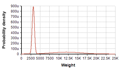 Distribution of vehicle weights

Another use arises when several situations are possible, but you don't know which situation you are in. If you have assessments for the uncertainty of a certain quantity for each situation, and you have an estimate for the probability of being in each situation, then the mixture of the distributions for each situation weighted by the probability gives your net uncertainty.
- Example: A stock trader knows that the FDA will soon be ruling on whether a certain company's new drug will be approved or not. He believes if it is approved, the companies stock price will see a change estimated at
Normal(180%, 40%), but if it is not approved he expects the price to change byNormal(-60%, 30%). Since he believes there to be a 50% probability of approval, an equally weighted mixture can be used to model the projected change in stock price.
Mixtures are also used when combining assessments from multiple experts. The assessment distributions from each expert can be mixed using a subjective weight reflecting each expert's credibility.
- The relative credibility of experts is not a precisely-defined quantity, although it is can still be employed without too much confusion in practice. An alternate interpretation is that you can one expert is "correct" and the other experts are wrong. Strictly speaking, this does not make sense, since an assessment is a subjective representation of uncertainty, not something that has a "correct" or "incorrect" answer. However, using this idea, you can interpret the weighting to be the probability of each expert being the correct one. The mathematics of combination are the same, it is just a metaphor for interpreting the weights.
When you are estimating uncertainty of a quantity, and you feel the uncertainty is bi-modal or multimodal, a mixture is usually the most direct and intuitive way to encode multimodal uncertainty. Most standard parametric distributions are unimodal (i.e., they have only one peak in the density graph), so you can't employ these alone.
Difference between a mixture and a sum
A mixture distribution is not the same as the distribution for the weighted sum of random variables.
- Example: There are 67 cars and 33 trucks on a road, with the weight of cars distributed as
Normal(3200, 300), and truck asNormal(12K, 4K). The distribution of total weight is show here (compare this to the distribution of vehicle weights above):
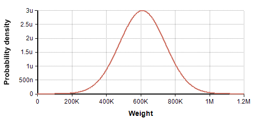 Uncertainty in the total weight of cars and trucks

This is not a mixture at all. In fact, it is a Normal distribution, and is quite distinct visually.
Encoding mixtures in Monte Carlo
In the most common case, you will encode the uncertainty in your chance variables and let Monte Carlo propagate the uncertainty for you. A mixture is NOT formed as the weighted sum of distribution functions. That would be encoding the distribution of the weighted sum (e.g., the total weight of cars and trucks).
A two component mixture is usually encoded using and IF-THEN-ELSE with a Bernoulli for the If clause, as in this example:
More generally, suppose you have an array of distributions, dists, indexed by I, and a vector of weights, wt, also indexed by I and which sum to 1. The mixture distribution is encoded as
ChanceDist(wt, dists, I)
Density and cumulative density of mixtures
Analytic density functions and cumulative density functions are formed from the component analytic density and cumulative density functions by weighted sums. So, for example, the analytic density at x of the cars and trucks mixture example is given by
0.67*DensNormal(x, 3200, 300) + 0.33*DensNormal(x, 12K, 4K)
and the cumulative density is
Enable comment auto-refresher