Tutorial: Open a model to browse

This chapter shows you how to:

• Open an existing model
• Calculate results
• Change input values to calculate different results

In this chapter, you use the Rent vs. Buy model, an Analytica model that compares the cost of renting a house to the cost of buying one. After working through the chapter, you will know how to open an existing model, use it to calculate results, and change input values to calculate different results.

Opening the Rent vs. Buy model

To begin, follow these steps.

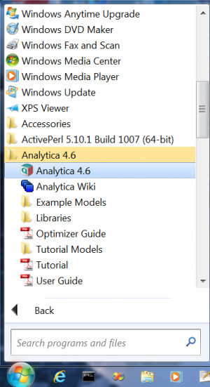
1. Launch Analytica: Click the Start button on the Windows taskbar. Click All Programs → Analytica 4.6 → Analytica 4.6.
   
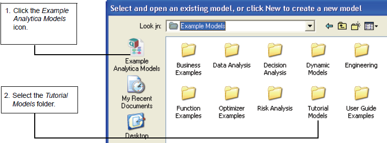
2. After Analytica starts, select File → Open from the menu.
3. Click the Example Analytica Models icon and select the Tutorial Models folder.
   
4. Open the Rent vs. Buy model.
5. Double-click the icon for the Rent vs. Buy model to start Analytica.
   
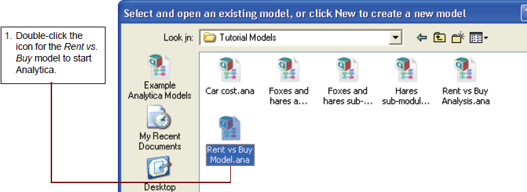
6. Analytica reads in the Rent vs. Buy model.

Becoming familiar with the Diagram window

When you open a model, Analytica first displays a top-level Diagram window. The Rent vs. Buy model diagram shows several input variables that affect the trade-offs between renting and buying, Normal buttons, a Calc button, and a node labeled Model.

This top-level diagram is an end-user interface to the model itself, which is contained in the Model node. In this chapter, you use only the interface in this top level diagram; in the following chapters you will explore the model in more depth.

Across the top of the screen is a horizontal palette of buttons. This is called the tools palette.

When you first open the Rent vs. Buy model, the browse tool is highlighted on the palette. With the browse tool selected, the cursor looks like a hand when it is over the diagram. The browse tool allows you to calculate the model, change input values, and examine — but not change — the structure of the model. In this chapter, you only use the browse tool.

Accessing Help Resources

At any time, you can press the F1 key on the keyboard or use the Help pull-down menu to access Analytica’s help resources. These include User Guide and Tutorial documents as well as Analytica’s online Wiki pages.

Computing output values

In the Rent vs. Buy model, the output value of interest is at the bottom, Present value of buying and renting.

Click the Calc button to compare the present value of buying and renting.

The output value displays in a Result window. This Result window shows a graph of two probability density curves, one for buying and one for renting. In a probability density graph, the units of the vertical scale are chosen so that the total area under each curve is 1 (100%). 25μ corresponds to 25 x 10-6 or 0.000025.

---

Numerical suffixes like μ and K are used extensively throughout Analytica. A quick reference for these suffixes is given on the back page of this tutorial.

---

Since the graph is of probability densities, both buying and renting have probabilistic, or uncertain, inputs. The probability density graph for each appear to be bell-shaped curves (normal distribution), although they appear a bit “noisy.”

The graphs show that the cost of renting, given the model’s inputs, are between about $105,000 and $155,000 (the negative numbers mean cost — cash flowing out), while the cost of buying is between $115,000 and a gain of $75,000.

Note: Your results can vary slightly, since the model is generating random inputs based on a normal distribution for the uncertainty of the rate of inflation and for the appreciation rate.

Click the model Diagram window to bring it to the front. Notice that the button next to Costs of buying and renting has changed to Result. The Result button indicates that the value has been computed; clicking the Result button re-displays the computed values.

Changing input values and recomputing

Now you will change some input values to the model and recompute the rent vs. buy comparison. You will change the values of Time horizon, Monthly rent, and Buying price.

Click the box next to Time horizon. Change the value to 7 and press Alt+Enter.

---

The main Enter key and the numeric keypad Enter key are not interchangeable. They have different functions in Analytica. Alt+Enter is equivalent to the numeric keypad Enter key.

---

As soon as you change an input, the Result button changes to a Calc button, indicating that Present value of buying and renting needs to be recomputed.

Click the box next to Monthly rent. Change the value to 1400 and press Alt+Enter.

Click the box next to Buying price. Change the value to 180K (or 180000) and press Alt+Enter.

Now you are ready to recompute to see the new results. Click the Calc button to compute the comparison of the costs of buying to renting.

The graphs show that the cost of renting, given these changed inputs, is between $90,000 and $120,000, while the cost of buying is between $135,000 and a gain of $70,000.